Finding critical points of a multivariable function

In the same way we have to rely on derivatives to find critical points of a single variable functions, we have to rely on partial derivatives to find critical points of a multivariable function. The idea of looking for points were we have horizontal tangent lines or zeroes of a function remains the same for multivariable functions. Except that for two variables we have a tangent plane, not just a single line.

Criteria do find critical points

Let [math]\displaystyle{ f }[/math] be a function with a domain [math]\displaystyle{ D }[/math]. [math]\displaystyle{ P_0 \in D }[/math] is a point of maximum or minimum. If [math]\displaystyle{ f }[/math] is differentiable at [math]\displaystyle{ P_0 }[/math], then its first order partial derivatives are equal to zero at that point.

With this theorem we can reduce our search for local maximums or minimums to points where we have partial derivatives equal to zero. Other points from the function's domain, not including the boundary, with partial derivatives different from zero, are automatically discarded from our search.

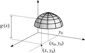
Suppose that [math]\displaystyle{ (x_0,y_0) }[/math] is a local maximum of [math]\displaystyle{ f }[/math]. With [math]\displaystyle{ (x_0,y_0) }[/math] being inside [math]\displaystyle{ D }[/math], excluding the boundary, there exists an open ball [math]\displaystyle{ B \subset D }[/math], centered at [math]\displaystyle{ (x_0,y_0) }[/math], such that, for all [math]\displaystyle{ (x,y) }[/math] in [math]\displaystyle{ B }[/math]:

[math]\displaystyle{ f(x,y) \leq f(x_0,y_0) }[/math]

On the other hand, there exists an open interval [math]\displaystyle{ I }[/math], with [math]\displaystyle{ x_0 \in I }[/math], such that for all [math]\displaystyle{ x \in I }[/math], [math]\displaystyle{ (x_0,y_0) \in B }[/math]. Let's consider the function [math]\displaystyle{ g }[/math] given by

[math]\displaystyle{ g(x) = f(x,y_0), \ x \in I }[/math]

If you didn't understand the single variable function [math]\displaystyle{ g }[/math], remember that we are keeping the other variable fixed, constant, like when we calculate partial derivatives.

We have:

• [math]\displaystyle{ g }[/math] is differentiable at [math]\displaystyle{ x_0 }[/math]
• [math]\displaystyle{ x_0 }[/math] is a point inside [math]\displaystyle{ I }[/math]
• [math]\displaystyle{ x_0 }[/math] is a point of local maximum of [math]\displaystyle{ g }[/math]

[math]\displaystyle{ g'(x_0) = \frac{\partial f}{\partial x}(x_0,y_0) = 0 }[/math]

We can repeat the same reasoning to prove that [math]\displaystyle{ \frac{\partial f}{\partial y}(x_0,y_0) = 0 }[/math]. We can also change the inequality sign to repeat the same proof, but for minimum points.

The geometrical interpretation of the proof is that we have an horizontal tangent plane at points where the function has a local maximum or minimum. It's a critical point and it can also be called a stationary point. We can resort to physics to explain the meaning of a stationary point. When we study trajectories, any object that is thrown upwards is going to be pulled back down by gravity, unless its velocity is above a certain value called the escape velocity. The exact moment when the vertical velocity vector changes its sign corresponds to a stationary point.

Note: I followed Hamilton Guidorizzi's proof.

The second derivative test

Continuing from the previous theorem, for [math]\displaystyle{ (x_0,y_0) }[/math] to be a local or relative maximum we have to have [math]\displaystyle{ \frac{\partial^2 f}{\partial x^2}(x_0,y_0) \leq 0 }[/math] and [math]\displaystyle{ \frac{\partial^2 f}{\partial y^2}(x_0,y_0) \leq 0 }[/math]. Invert the inequality sign and we have a condition for a point to be a local or relative minimum.

The geometrical interpretation is pretty much the same that we had for single variable functions. The second partial derivative is about the concavity in one direction. When they are both negative, concavity is downwards for both directions. When they are both positive, concavity is upwards for both directions. We can already go further and state that if the sign of each second order partial derivative is the opposite of the other, that's a saddle point. The equivalent to an inflection point for single variable functions.

The reasoning for this proof is pretty much the same that we did for single variable functions. Except that the second order derivative is now a partial derivative.

Most textbooks give the definition of the Hessian:

[math]\displaystyle{ H(x,y) = \left| \begin{matrix} \frac{\partial^2 f}{\partial x^2} & \frac{\partial^2 f}{\partial xy} \\ \frac{\partial^2 f}{\partial yx} & \frac{\partial^2 f}{\partial y^2} \end{matrix} \right| = \frac{\partial^2 f}{\partial x^2} \frac{\partial^2 f}{\partial y^2} - \frac{\partial^2 f}{\partial xy} \frac{\partial^2 f}{\partial yx} }[/math]

The conditions for a local maximum or a local minimum should have been made clear in the previous paragraph. Let's move to the saddle point:

If [math]\displaystyle{ H \lt 0 }[/math] we have a saddle point. From the Hessian's formula we have that it's negative when the first term is less than the second.

Another point of view is to think on the Hessian as a dot product between two vectors. It does resemble the directional derivative.

If [math]\displaystyle{ H = 0 }[/math] we cannot state anything about that point because we have the same issue with single variable functions. The second derivative can give us information about the function's concavity if the derivative is different from zero. When it's equal to zero we can't know for sure.